Assessing the metabolic burden of a DNA construct on the host, a first draft

Phew it’s been a while! I’ve been busy, but in all honesty I haven’t done a Transcriptic blog recently because I’ve been doing a lot of repetition trying to optimise plating bacteria. There’s a lot to write about, but I think it would be best for both you and I if I try and keep it short. In this post I want to cover doing some rough analysis of early data from my burden assay project on Transcriptic.

First up, some house keeping. I’m going to be in the bay area July 21 to 31 so say hi to me on twitter if you want to grab a coffee/pint and talk biotech/startups/science etc.

Burden Assay

OK so this assay assesses the metabolic burden inflicted upon a bacterium by a synthetic construct. Metabolic burden has huge implications for industrial scale biotech in applications such as the production of recombinant proteins or other bioproducts such as farnesene used in the fine chemical industry. High metabolic burdens can result in poor yields of the target product or an unsustainable process. With this in mind an assay that enables the assessment of metabolic burden becomes a tool for screening different constructs to minimise burden whilst maximising yield.

This burden assay comes from Ellis et al. at Imperial College London. You can read the full paper on bioRXiv and watch an awesome PLOS Syn Bio community hangout below. I recommend watching the video for background on this assay because I don’t go into it too much in this post.

I attempted to replicate the burden assay protocol on Transcriptic and Tom Ellis and his group very kindly provided me with the strains that possess the genomic burden reporter.

Results

Colonies

In the experiment I plated 3 different samples, 50µL of: strain M1 at 0.01% v/v dilution, strain M1 at 0.1% v/v dilution and strain pSB1C3 at 0.01% v/v dilution. These concentrations were determined through a prior experiment where serial dilutions of a strain were made and 6 different concentrations plated to see which concentration gave rise to the most colonies.

The concentrations are quite low, this is because when the strains were shipped to Transcriptic they reached OD600 readings just above 1. This is pretty messy and settling on a known volume of a known OD600 would make this more repeatable.

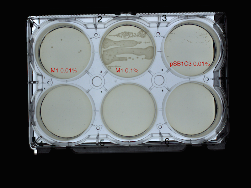Fig. 1 - M1 and pSB1C3 plated on LB-agar and incubated at 37 celsius for 14 hours.

|Well|Colonies Picked| |:—-:|:—————:| |A1|4| |A2|5| |A3|8| Table 1 - Colonies picked by autopick() for each well, unfortunately a difficult to control process.

In the protocol, up to 8 colonies are picked for each sample. 3 colonies from each sample were specified as the test group and the remaining colonies were used as negative controls. This design unfortunately means that while all 3 samples had 3 replicates, M1 0.01% only had 1 negative control while pSB1C3 0.01% had 5 negative controls. I need to nail picking 8 colonies consistently.

The picked colonies innoculate separate wells where the strains are cultured, then eventually added to the assay plate. Here the spectroscopic time series begins where 24 fluorescent measurements of GFP and RFP are taken alongside OD600 measurements with 30 minute incubation periods in between each measurement. After the first hour in the time series the sample group is supplemented with arabinose an inducer for the construct, where as the negative controls remain uninduced.

Spectroscopic time series

After the run was complete I wrote some R code to do the curve plotting.

require('jsonlite')
require('httr')
require('dplyr')
require('tidyr')
require('lubridate')
require('dotenv')

load_dot_env('.env')

substrRight <- function(x, n){
  substr(x, nchar(x)-n+1, nchar(x))
}

email <- Sys.getenv("TRANSCRIPTIC_USER_EMAIL")
token <- Sys.getenv("TRANSCRIPTIC_API_TOKEN")

url <- Sys.getenv("TRANSCRIPTIC_DATA_URL")
req <- GET(url, config(httpheader = c("X-User-Email" = email, "X-User-Token" = token)))

## GET data from Transcriptic
json <- content(req, as = "text")
df <- fromJSON(json)

## Remove non spectroscopic data such as colonies picked
for ( i in 1:4) {
  df[1] <- NULL
}

Above is the setup for the analysis code, it shows the use of jsonlite and httr to fetch the data from the Transcriptic API and parse the JSON into a dataframe. The end of the snippet shows a for loop that just goes through non-spectroscopic data and deletes it.

The following snippet shows the extraction of both spectroscopic and timing data from the parsed API response. The timing data is used to create an elapsed time in seconds from the first spectroscopic measurement.

# Extract the spectroscopic data.
speclist <- data.frame(t(sapply(df, "[[", "data")))
# Extract the executed_at timestamp from the run data.
exectime <- data.frame(t(sapply(df, "[[", "instruction"))) %>% select(executed_at)
# combine the spectroscopic data and the timing data
specdf <- data.frame(speclist, exectime)
specdf<- data.frame(sapply(specdf, function(x) unlist(x)))

specdf <- cbind(dataref = rownames(specdf), specdf)
rownames(specdf) <- NULL

## Tidy - get everything into a 'tidy' data format
tidyspec <- gather(specdf, "well", "abs",
  a1:b1:c1:d1:e1:f1:g1:h1:
  a2:b2:c2:d2:e2:f2:g2:h2:
  a3:b3:c3:d3:e3:f3:g3:h3)
## Mod calculate the elapsed time for the time series data by using the oldest time as t zero
start_time <- tidyspec %>% summarise(min(executed_at))
tidyelapse <- tidyspec %>%
  mutate(elapsed = ymd_hms(executed_at) - ymd_hms(start_time))

Here are the growth curves, showing OD600 absorbance units, green fluorescence and red fluorescence in arbitrary units and the x-axis is elapsed time in hours. Sorry the graphs aren’t labelled nicely, it was a pretty rough first draft at analysis.

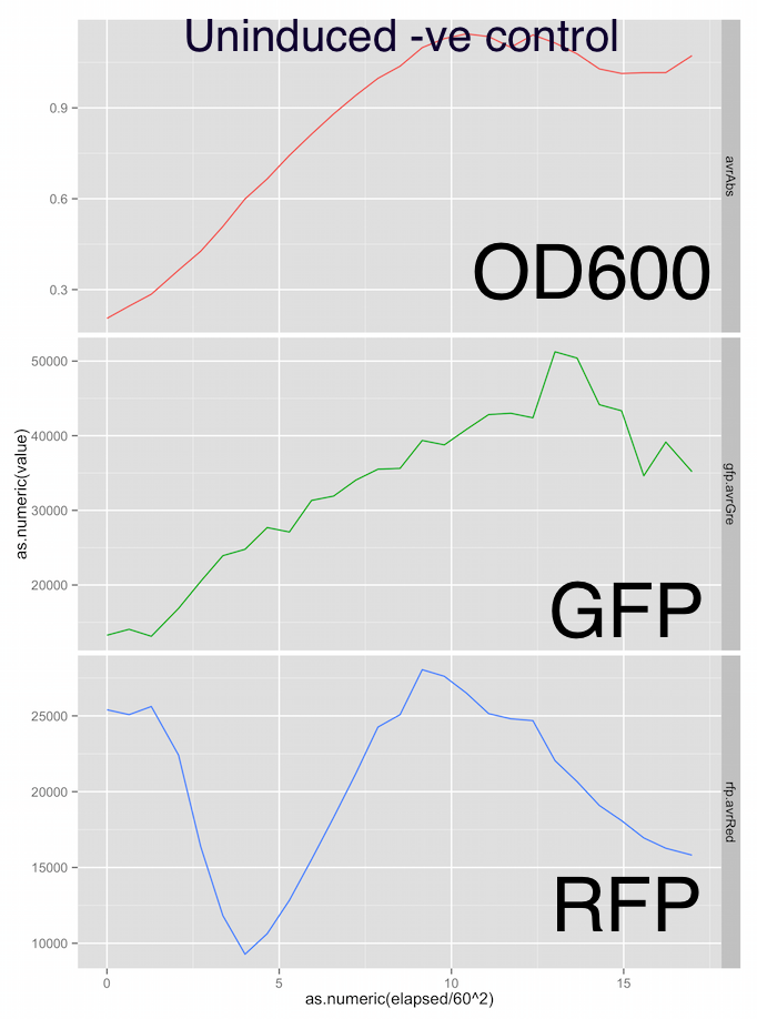Fig. 2 - Uninduced M1 strain shows a typical OD600 growth curve for E. Coli and the increase in GFP output (constituitively expressed) coincides with growth, suggesting no metabolic burden.

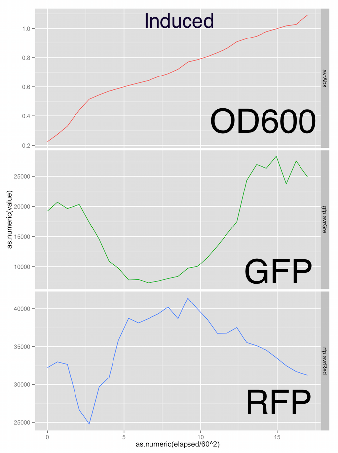Fig. 3 - Induced M1 strain shows a suppressed growth rate relative to the negative control. GFP output appears massively reduced, indicating there is a metabolic burden on the bacteria due to the construct being induced by arabinose.

The RFP fluorescent output in both the test and control groups is a little all over the place. However the test group RFP output peaks at 40,000 vs the 25,000 of the negative control group. I’m not relly trusting the RFP channel at the moment.

Conclusions

The expected metabolic burden was present in the test group indicated by a suppressed growth rate and massively suppressed GFP output relative to the negative control group. This is really promising for a first attempt at this assay.

Comments

There were actually some problems with this run. I didn’t take into account mandated disposal volumes required by Transcriptic for performing pipette transfers. This actually resulted in some wells of the assay plate, not receiving fructose therefore the media was devoid of any carbon source. I have updated the protocol to hopefully fix this issue.

What’s great is now that first draft is established for both the run code and the analysis code I should be able to get into a nice iterative cycle of improvement for this assay with far less time than it would require to do in person in the lab!

That actually turned into a huge post, sorry! I hope you found it interesting.

Special thanks to Tom Ellis and Francesca Ceroni from Imperial College and Taylor Murphy from Transcriptic who have all been very helpful and patient with me.